Institute of Mechanics, Chinese Academy of Sciences
Keywords: flow visualization, laser-induced fluorescence
Fluid mechanics is a branch of mechanics that primarily studies fluids at rest and in motion under various forces, as well as their interactions and flow behavior when fluids and solid boundaries move relative to one another [1]. The air all around us is an important subject of fluid-mechanics research. From bicycle helmets and biomimetic aircraft to supersonic planes, whenever an object is within Earth’s atmosphere and either flying or moving rapidly through it, fluid-mechanics problems will inevitably arise. Computational fluid dynamics (CFD) is an important tool for studying fluid-mechanics phenomena and designing aerodynamic shapes. However, in combustion processes involving chemical reactions, or in hypersonic flight where the ideal-gas model no longer applies, there is still a need for many experiments to study various problems.
Measuring data is an important part of experiments. Optical diagnostics use certain optical properties of a flow field to measure its parameters. The technique has distinctive advantages: it causes virtually no disturbance to the mechanical properties of the flow and responds very quickly. With laser light sources, which have high energy density and good monochromaticity, the signal-to-noise ratio of measurements can be greatly improved and specific flow information obtained. Laser-induced fluorescence (LIF) inherits these advantages, in addition, it can obtain the spatial distribution of flow information, making it an important means of visualizing flow.
As its name suggests, laser-induced fluorescence is a measurement method in which researchers use a laser to excite particles in a flow field to high-energy quantum states, then detect the fluorescent photons they emit. Fluorescence is a form of cold light emission produced by photoexcitation. As shown in Figure 1, when fluorescent particles are illuminated with suitable light, there is a certain probability that they will absorb photons and transition to an excited state, then immediately relax to a lower energy level and emit photons. The energies of the absorbed and emitted photons correspond to the differences between the energy levels involved in these transitions, so each fluorescent substance has relatively well-defined wavelength ranges for absorption and emission. In common Stokes fluorescence, the emitted photon typically has lower energy than the excitation photon, so the fluorescence wavelength is usually longer than the excitation wavelength. The wavelength difference between the peaks of the excitation and emission spectra is called the Stokes shift. Once illumination stops, the fluorescence process also ends within 1 microsecond. A familiar everyday example is using ultraviolet light on a banknote to make its security features emit fluorescence visible to the human eye.
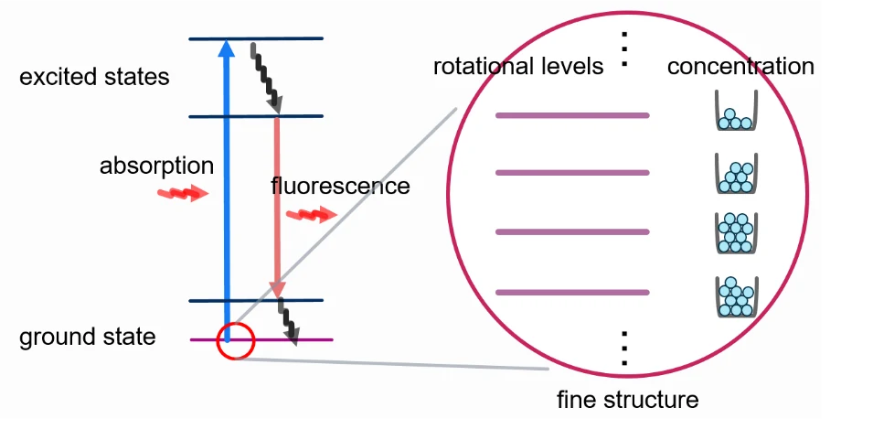
Figure 1: The principle of fluorescence generation
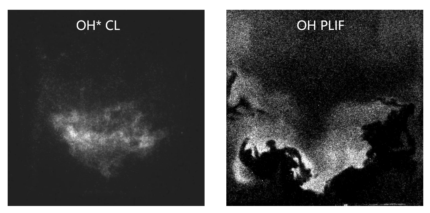
In many applications, we use a laser sheet to illuminate a flow field and induce fluorescence from species such as OH radicals. A camera then records the fluorescence distribution in that plane, providing two-dimensional flow information [2]. OH radicals are important intermediates in the combustion of alkane fuels and are widely distributed in flame reaction zones and high-temperature combustion products. Figure 2 shows images of OH radical chemiluminescence—light produced by combustion itself—and OH planar laser-induced fluorescence in a flame. The chemiluminescent region is three-dimensional, and the camera records the sum of all light along the line of sight. Laser-induced fluorescence, however, clearly reveals the distribution of OH radicals inside the flame, enabling precise flow visualization. Common fluorescent species in gaseous environments include combustion intermediates such as OH, CH, and CH2O, the major combustion pollutant NO, kerosene fuel molecules, and others. Depending on the application, fluorescent species can also be other molecules, metal atoms, or ions in a plasma.
Figure 2: Comparison of OH* chemiluminescence photography (left) and OH planar laser-induced fluorescence (right)
The signal intensity of laser-induced fluorescence is closely related to laser parameters and the concentration of the fluorescent species. It is also markedly affected by temperature, pressure, other quenching species, and additional factors. Consequently, determining species concentrations with this technique requires several steps. For the same reason, laser-induced fluorescence can also be used to infer temperature and velocity distributions in a flow field. Commercial dye lasers can resolve the rotational energy levels of NO molecules and OH radicals. Comparing the fluorescence efficiencies of two different energy levels of the same species allows the flow temperature to be inferred [3]. In hypersonic flow, the spectral lines of rapidly moving fluorescent molecules undergo noticeable Doppler shifts, which can be used to infer the velocity component parallel to the laser direction [4]. Alternatively, a high-power ultraviolet laser can dissociate larger molecules into commonly used fluorescent molecules, marking the flow. After letting these molecules travel for a short time, imaging them with laser-induced fluorescence gives the displacement of the marked line, allowing the velocity component perpendicular to the laser direction to be calculated [5].
Because light sources used for laser-induced fluorescence are mainly in the ultraviolet range, commercial dye lasers are currently the most commonly used lasers. The cover image shows the dye laser used for NO laser-induced fluorescence. Compared with infrared semiconductor lasers, they require much more space and maintenance expenditure. Nevertheless, to study turbulent flames more thoroughly, scientists have combined multiple lasers to monitor fluorescence from several species simultaneously, together with techniques such as particle image velocimetry (PIV) [6,7], to investigate the effects of turbulence on flame fronts.
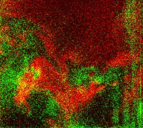
Figure 3: Planar laser-induced fluorescence images of OH (red) and CH2O (green)
*This article represents the authors’ personal views and does not represent the views of this website. Other media, websites, or individuals reusing or republishing it must acknowledge the source and assume responsibility for copyright and other legal matters. Authors who do not wish to have their work republished, or who wish to discuss remuneration or other republication matters, should contact us.
References:
[1] Baidu Baike: Fluid mechanics
[2] Hanson, R.K., Seitzman, J.M., and Paul, P.H. Planar Laser-Fluorescence Imaging of Combustion Gases. Appl. Phys. B 50, 441-454 (1990)
[3] Wollenhaupt, M., Rosenhauer, M., M¨uller, et al. NO laser-induced fluorescence studies for the application of single-shot two-line thermometry to HEG. 21st International Symposium on Shock Waves, Great Keppel Island, Australia, July 20-25, 8360 (1997)
[4] Palmer, J. L. and Hanson,R.K. Single-Shot Velocimetry Using Planar Laser-Induced Fluorescence Imaging Of Nitric Oxide. 29th Joint Propulsion Conference and Exhibit. June 28-30, 1993 / Monterev, CA
[5] Wehrmeyer, J.A., Ribarov, L.A., Oguss, D.A., et al. Flame Flow Tagging Velocimetry with 193-nm H2O Photodissociation. Appl. Opt. 38, 6912–6917 (1999)
[6] Li, Z. S., Li, B., Sun, Z. W., et al. Turbulence and combus-tion interaction: High resolution local flame front struc-ture visualization using simultaneous single-shot PLIF imaging of CH, OH, and CH2O in a piloted premixed jet flame. Combustion and Flame, 2010, 157(6):1087–1096.
[7] Watson, K. A., Lyons, K. M. Scalar and velocity field measurements in a lifted CH4–Air diffusion flame. Combustion and Flame, 1999, 117(1/2):257–271.
Sources for this revision: Thermo Fisher Scientific · Anatomy of Fluorescence Spectra.
Sources and editorial history
Editorial revision note: On October 10, 2026, the direction of the Stokes-shift wavelength change was corrected by comparison with the original website article and a fluorescence textbook. The original author and publication record are retained.